Calculating Percent Change Between Rows in SQL
Track changes between rows in ordered SQL data using window functions


When working with time-based data or data sorted in a specific order, you often need to compare each value to the one before it. This comes up when tracking changes in prices, counts, or totals over time. One way to measure those changes is by calculating the percent difference from one row to the next. Doing that in SQL takes more than basic subtraction and division because SQL works with sets, not rows one at a time. To compare values across rows, you need functions that let you look at a previous value while keeping the overall data grouped and sorted the way you need it.
Comparing Rows Using Window Functions
Most SQL queries return one row at a time in the result, but they don’t process one row at a time the way a script does. SQL works with whole sets at once. So when you want to compare each row to the one that came before it, that’s not something SQL does automatically. You have to be very specific about how the data should be ordered, and how one row relates to another. Without giving SQL a rule to follow, it won’t know what “previous” means. That’s where window functions come in.
Window functions are built for working across rows while still returning one result per row. When they run, they don’t change the number of rows, but they let you reach into nearby rows in a defined order. You can grab values from earlier or later rows in the same result. That’s what lets you build comparisons like “this number compared to the one before it.”
Let’s look closer at what SQL is doing in the background and how the LAG() function fits into it.
What SQL Actually Does When You Query
When you send a query that uses a window function, SQL evaluates it in stages. First it applies filters like WHERE. Then it gathers and orders the rows you’ve asked for. When you use something like LAG() or LEAD(), SQL doesn’t reorder the rows in your table. It just applies the function based on the ordering you tell it to use inside the OVER() clause. If you don’t include an ORDER BY in your window function, there’s no guarantee about the direction it compares. SQL will still run, but the results can be unpredictable. That means ordering is a required part of the logic, not just a formatting step.
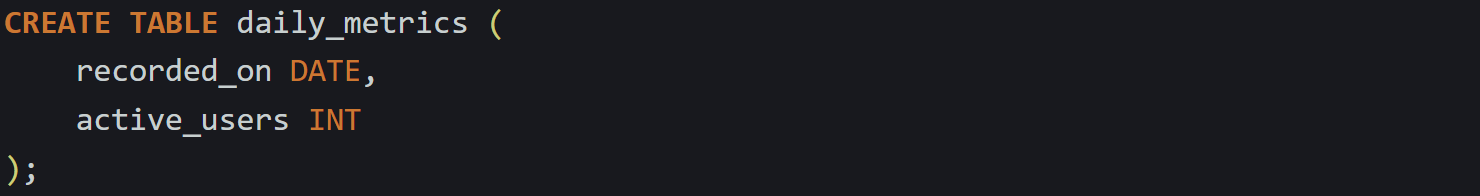
Let’s say you have a table tracking the number of active users per day:
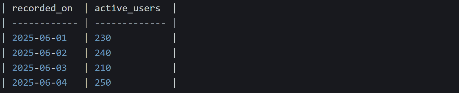
And this data is in the table:
If you want to compare each day’s number to the day before, your instinct might be to try some kind of self-join, but that gets messy fast. A window function gives you a way to do it cleanly without reshaping your query structure.
Here’s a query that adds a column showing the previous day’s user count:
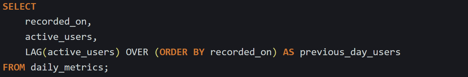
This works because LAG() uses the order given in the query to decide which row comes before. It does not follow the physical order of the table or make any assumptions.
The Mechanics Behind LAG
The LAG() function is part of a group of window functions that give access to other rows without changing the number of rows returned. You can use it to look behind, or use LEAD() to look ahead. The structure is:

column_nameis the value you want to pull from another rowoffsetis how many rows back you want to look (defaults to 1 if you skip it)defaultis what to return if there’s no previous row (optional)
In most cases where you’re tracking changes, you just want to look one row back. Here’s a quick breakdown with some variations:
Basic one-row-back

Same as:

Looking two rows back

This shifts the window further back. Useful if you want to compare with more distance, such as two days ago.
Supplying a default

This avoids a NULL in the first row. But be careful. If you're going to divide by this value later, and it’s zero, it can cause errors. You can’t use LAG() without OVER. And you can’t use OVER without giving it something to order by, at least in this case. The ordering is what tells SQL how to move through the data. Without it, LAG() has no direction.
If you need to apply this logic to different groups of data inside the same table, like multiple users or multiple stores, you can use a partition to keep the comparisons inside each group. That’s done by adding PARTITION BY before the ORDER BY.

Now the function only looks back within each store_id group, which keeps comparisons accurate across separate timelines.
The way LAG() and other window functions are processed lets you stack them without needing nested queries. That makes it easier to compare, rank, or measure trends directly inside a single pass. Window functions are evaluated after FROM, WHERE, GROUP BY, and HAVING but before the final SELECT list and any ORDER BY. That timing lets them read any column in scope for SELECT. When you understand how that timing works, it opens the door to more flexible queries.
How Percent Change Works and How SQL Gets There
Once you have access to the previous row using LAG(), the next step is to actually measure the difference between the current row and the one before it. In time-based reports or trend summaries, raw numbers only show part of the picture. Percent change helps you measure movement relative to size. A jump from 5 to 10 is bigger than a jump from 100 to 105, even though both increased by 5. So instead of focusing on just the absolute change, you divide that change by the previous value to get a percent.
To do this with SQL, you combine LAG() with math inside the SELECT statement. SQL doesn't have a built-in percent change function, but it's just basic arithmetic. The only extra work is making sure you handle data types and missing values correctly.
The Math Of Percent Change
The formula you’re using here is the same one used in spreadsheets and analytics tools:

That gives you a percentage representing the change from the previous value. If the result is positive, it increased. If it’s negative, it decreased.
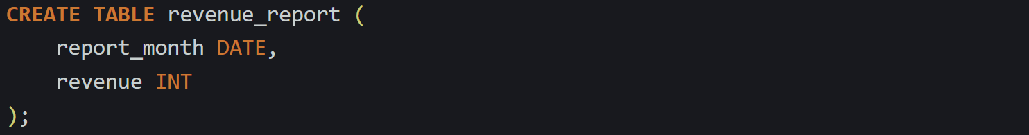
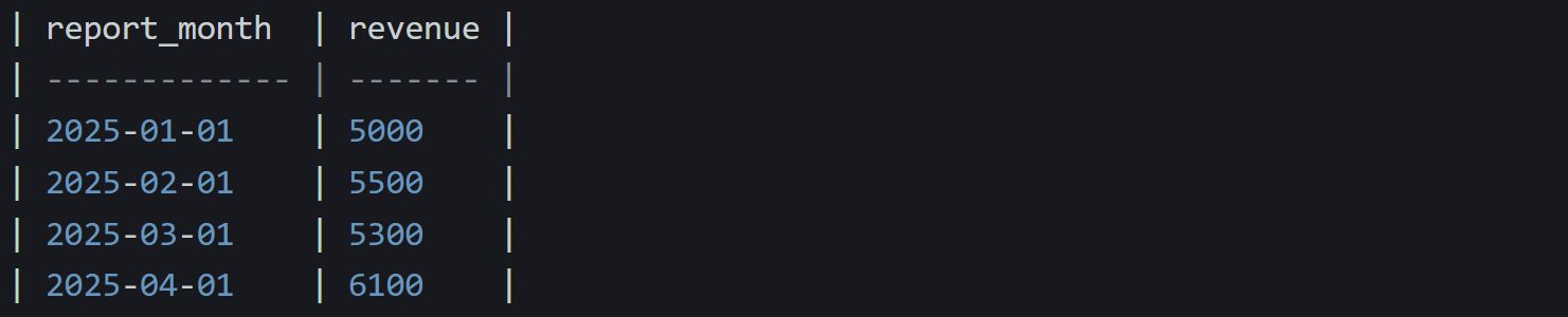
Let’s say you’re working with monthly revenue data:
And it has rows like this:
You already know how to get the previous row’s value using LAG():

To get the percent change, you subtract the lagged value from the current row’s revenue, divide that difference by the lagged value, and multiply by 100. You’ll also want to cast at least one part of the math to a decimal-friendly type like FLOAT, or SQL might round too early if both numbers are integers.
Here’s the full query:
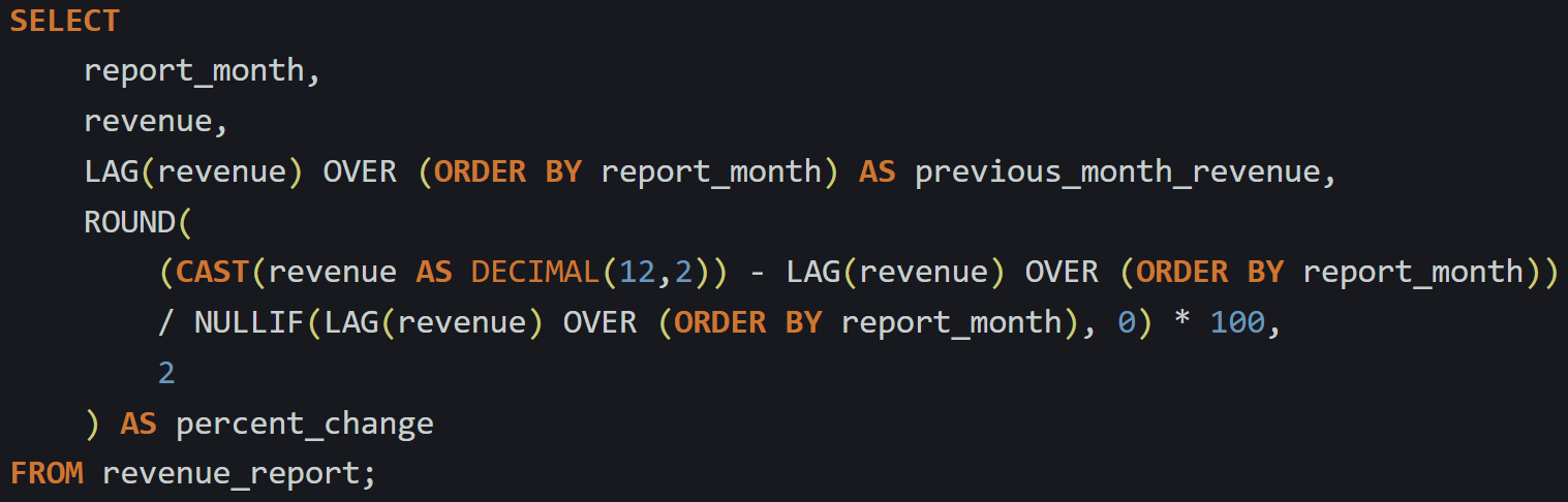
This gives you the percent change column right next to your data. You’ll notice LAG(revenue) is repeated in two places, which can be a little heavy. Most planners reuse the window result internally, but repeating the expression hurts readability, so moving it into a CTE keeps the statement cleaner.
A Smoother Version With A Common Table Expression
To avoid calling the same LAG() function multiple times, it helps to move that logic into a temporary result set first. That way, the lagged value is only calculated once and can be reused.
This is where a common table expression, or WITH block, makes the query easier to follow.
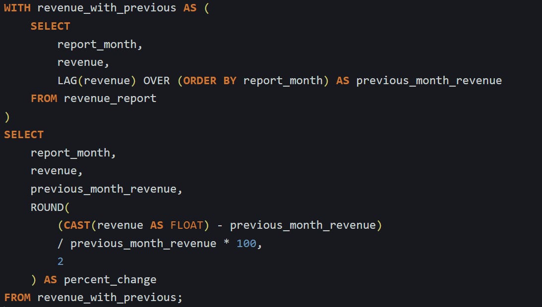
This version improves clarity and avoids repeating the same function. You’re still using the same formula, but now the percent change can read directly from previous_month_revenue instead of recalculating it each time. The cast to FLOAT is still necessary to preserve decimals, especially if you want to avoid a long chain of rounding and truncation. The result looks more readable, and the logic becomes easier to update if anything changes.
What Happens When Previous Row Is Missing
There’s one detail that always comes up when you use LAG() for comparisons. The very first row in any ordered result has no previous row to compare against. When there’s no previous value, LAG() returns NULL. This happens by design. And that affects your percent change. Once a NULL is in the mix, the whole expression becomes NULL. So your first row won’t have a percent change value. That’s usually what you want. But you have a couple of options if you need to control it more directly.
You could supply a default value using the third argument in LAG():

That replaces NULL with zero. But that comes with a catch. Dividing by zero will break the query, so you’ll still need a safety check. It’s better to leave the default as NULL and then write a condition that handles it.
You can add a conditional block inside your SELECT:
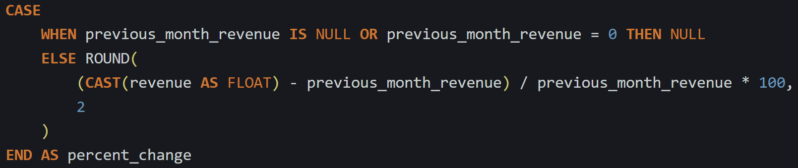
This adds a check for both NULL and zero. If the previous value is missing or zero, the percent change will be NULL, which is safer than having the query fail.
Even though it adds more code, this kind of control matters in reports where accuracy and stability matter. You don’t want the whole query breaking because the first row had nothing to compare against. With this in place, your output will be consistent and readable without surprises.
Conclusion
SQL works by processing data in ordered sets, not as individual steps from top to bottom. That’s what makes window functions like LAG() possible. They let you reference a nearby row without flattening or reshaping the structure. When paired with basic math, they give you a way to measure change across rows while keeping the query clean and set-based. With the right ordering and a clear check for missing values, you can get accurate percent comparisons that match how trends move over time.