

Cycles in linked lists show up in real work more than most expect, from network structures that loop back on themselves to data nodes that accidentally form a ring. A cycle happens when a node connects to one that came before it, creating an endless loop during traversal. Floyd’s Cycle Detection Algorithm, also called the Tortoise and Hare method, gives a reliable way to spot those loops without extra memory. It depends on two pointers that travel at different speeds, meeting at a shared node if a cycle exists. Beyond finding the loop, it can also reveal the exact node where the cycle starts.
How Floyd’s Cycle Detection Works
Floyd’s Cycle Detection Algorithm builds on a simple idea that’s easy to miss at first. Two pointers travel through the same linked list at different speeds, one slower and one faster. If the list contains a cycle, the faster pointer will eventually catch up to the slower one within that loop. That single meeting point confirms that a cycle exists, even though neither pointer keeps track of previously visited nodes. What makes this method special is that it finds the loop without extra memory, which keeps it efficient for both small and large linked structures.
Slow and Fast Pointers Explained
The slow pointer moves one node at a time, taking the direct path through the list. The fast pointer moves two nodes at a time, covering twice the distance in each step. Both start from the same head node, and as they move, their relative distance changes. If there’s no loop, the fast pointer will eventually reach the end of the list. If there is a loop, the fast pointer will circle back and meet the slow one.
That cycle of motion can be seen through a simple structure like this:
 { this.data = data; this.next = null; } } public class CycleCheck { public static boolean detectCycle(Node head) { if (head == null) return false; Node slow = head; Node fast = head; while (fast != null && fast.next != null) { slow = slow.next; fast = fast.next.next; if (slow == fast) { return true; } } return false; } }")
The logic here keeps the space footprint constant while handling lists of any length. A cycle triggers a meeting between the pointers because their speeds differ. If both pointers move one node per step and start at the same head, they’re equal at every step, which makes detection meaningless. If they start at different nodes, they only meet when the initial offset is a multiple of the cycle length.
To understand this better, one of the easiest things to imagine two people running laps around a track. If one jogs slowly and the other sprints, the faster one will eventually lap the slower one. That same concept applies here, if the list loops the fast pointer will catch up from behind, confirming the presence of a cycle.
Changing the fast pointer to jump three nodes per step still detects cycles for any loop length. It only alters how long it takes to meet. Two steps remain standard because it keeps code simple and meeting time short.
 { if (head == null) return false; Node slow = head; Node fast = head; while (fast != null && fast.next != null && fast.next.next != null) { slow = slow.next; fast = fast.next.next.next; if (slow == fast) { return true; } } return false; }")
This variation still works. The meeting time inside a loop of length L advances by k − 1 per step, so with a three-step fast pointer (k = 3) the meet occurs after L / gcd(L, 2) steps. Most implementations usually keep the two-step version for readability.
Why the Meeting Point Matters
When the slow and fast pointers meet, the meeting itself proves that a cycle exists. It’s not random that they collide, their relative motion guarantees it inside a loop. The slow pointer always trails behind, while the fast one wraps around until they’re both aligned on the same node. That point of contact happens somewhere inside the cycle, though not necessarily where it begins.
Making sense of the math behind their meeting gives a better sense of how it works. Let’s call the distance from the list’s start to the cycle’s first node A, the distance from that node to the meeting point B, and the full length of the loop C. The slow pointer covers A + B steps, while the fast one travels A + B + nC, where n is the number of times it’s looped around. Because the fast pointer moves twice as fast, the equation becomes:
 = A + B + nC A + B = nC A = nC - B")
That simple relationship explains why the meeting is guaranteed. The difference in distance traveled aligns them in the loop after a whole number of cycles.
Here’s a compact way to print the step counts for both pointers, which helps visualize their progress as they move:
 { Node slow = head; Node fast = head; int step = 0; while (fast != null && fast.next != null) { slow = slow.next; fast = fast.next.next; step++; System.out.println(\"Step \" + step + \": slow=\" + slow.data + \", fast=\" + fast.data); if (slow == fast) { System.out.println(\"Meeting point at node \" + slow.data); return; } } System.out.println(\"No cycle detected\"); }")
Running this on a list with a loop gives an easy-to-read trace of both pointers and confirms exactly when they meet. It’s a quick test to verify how their speeds relate and how quickly they synchronize inside a cycle.
That meeting doesn’t only prove there’s a loop, it also sets the stage for finding where it starts, which comes next in the logic. Before getting there, it helps to pause and see that the method’s reliability comes from stable movement and simple math. The fast pointer keeps gaining ground with every step until the gap between the two equals a multiple of the loop’s length. At that moment, they land on the same node, confirming that the list circles back on itself.
Finding the Start of the Cycle
Detecting a cycle is only half the story. Once it’s confirmed that a loop exists, the next question is where it begins. Finding that starting point turns out to be as elegant as the detection itself, relying on the same two-pointer system. Floyd’s algorithm cleverly reuses what’s already known from the meeting point, applying a bit of distance logic to locate the exact node where the cycle starts.
Resetting One Pointer
After the slow and fast pointers meet inside the loop, one of them is reset back to the head of the linked list. The other stays at the meeting point. From there, both move forward one node at a time. Because of how their movements line up mathematically, they’ll eventually meet again at the cycle’s entry node. That point marks where the list starts looping back on itself.
The reasoning goes back to the distance equation. If the distance from the head to the start of the cycle is A, and the meeting happened B nodes into the cycle, then we know from the earlier math that A = nC minus B, where C is the total length of the cycle and n is the number of loops the fast pointer made. That means moving both one step at a time from those two positions will land them on the same node after A moves.
This method naturally fits how the pointers behave. The slow pointer at the meeting point is already B steps into the cycle, while the reset pointer needs to cover A steps. As they move together, they sync up perfectly at the cycle’s start.
To see this in practice, let’s imagine we have a linked list with values [10 → 20 → 30 → 40 → 50 → 30]. After detection, resetting one pointer to 10 while leaving the other at the meeting node inside the loop causes both to meet again at 30. That node is the cycle’s entry point.
It’s worth noting that the same logic works no matter how long the cycle is or how deep into the list it begins. The only difference is how many steps it takes before both pointers align.
Visualizing the Movement
Visualizing the movement of the pointers helps make the reasoning concrete. The fast pointer spends its early time looping while the slow pointer crawls forward, but once the reset happens, both move together at the same pace. From that moment on, their positions mirror one another in distance to the cycle’s start.
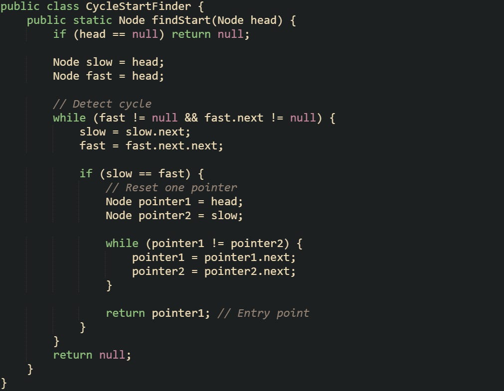
You can make the behavior more visible by tracking their positions as the algorithm runs. This next code example expands the earlier logic to print each movement step for both pointers:
 { Node slow = head; Node fast = head; while (fast != null && fast.next != null) { slow = slow.next; fast = fast.next.next; if (slow == fast) { Node pointer1 = head; Node pointer2 = slow; while (pointer1 != pointer2) { System.out.println(\"Pointer1 at \" + pointer1.data + \", Pointer2 at \" + pointer2.data); pointer1 = pointer1.next; pointer2 = pointer2.next; } System.out.println(\"Cycle starts at node \" + pointer1.data); return; } } System.out.println(\"No cycle found\"); }")
This trace confirms how the two pointers travel step by step and where they eventually meet again. It’s a good diagnostic tool for verifying the behavior of linked structures in tests or interviews.
For larger linked lists, cycles might start deep into the sequence, which can make visual debugging difficult. To help with that, you can adapt the logic to print only specific checkpoints or stop after a set number of moves to avoid infinite prints during early testing.
 { Node slow = head; Node fast = head; int moves = 0; while (fast != null && fast.next != null && moves < limit) { slow = slow.next; fast = fast.next.next; moves++; System.out.println(\"Move \" + moves + \": slow=\" + slow.data + \", fast=\" + fast.data); if (slow == fast) { System.out.println(\"Cycle detected at move \" + moves); return; } } System.out.println(\"No cycle detected within move limit\"); }")
Adding a step counter is a helpful way to watch pointer movement without getting stuck in an infinite loop. It’s particularly useful during debugging or classroom explanations where watching pointer travel clarifies how they align in real time.
Handling Edge Cases
Cycle detection works smoothly for most lists, but a few edge cases need to be handled carefully to avoid incorrect results or null references. For detectCycle on an empty list return false. For findStart on an empty list return null. A single-node list without a self-reference is not cyclical, so the same rule applies. If that single node links back to itself, the algorithm should correctly identify the head as both the meeting point and the cycle start.
This small helper version tests those edge cases to confirm the logic behaves as expected:
 { Node single = new Node(5); System.out.println(findStart(single)); // null, no cycle Node selfLoop = new Node(7); selfLoop.next = selfLoop; System.out.println(findStart(selfLoop).data); // 7, cycle starts at itself Node empty = null; System.out.println(findStart(empty)); // null, empty list }")
Each of these examples proves that Floyd’s algorithm holds consistent across small, minimal structures. It handles null inputs gracefully, doesn’t throw exceptions, and behaves predictably for every edge case.
Some developers also test cycles that start far from the head, such as after several nodes. Those tests confirm that distance doesn’t change correctness, only the number of steps taken before alignment. As long as the pointers move at one and two steps respectively, the cycle’s entry node will always be found accurately.
Conclusion
Floyd’s Cycle Detection Algorithm works through motion and timing inside a looped list. Two pointers move at different speeds, revealing a cycle when they meet. That same difference in pace helps find where the loop begins. The entire process runs on basic math and consistent movement rather than extra storage or complex structures. Its strength comes from how predictable it is, turning what could be a tricky problem into a reliable mechanical process that continues to fit modern Java development perfectly.
Brillaint breakdown of the tortoise and hare approach. The part about resetting one pointer to find hte cycle's start is especially clever since it directly leverages that A = nC - B relationship. I ran into a similar issue debugging a graph traversal where nodes accidentally linked back, and knowing this saved me from implementing a hash set. Would be intresting to see how this compares to Brent's algorithm for longer cycles.