

Working with data frequently calls for smoothing out daily noise so longer patterns stand out. A rolling average makes that possible by taking the mean over a fixed number of recent days. A common choice is the 7-day average, which balances how fast trends react with how steady they look. It’s used in business reports, financial tracking, and public health dashboards. The mechanics of calculating it in SQL depend on window functions that look across rows in relation to the current one.
The Basics of a Rolling 7 Day Average
A rolling average is one of the first tools people reach for when they need to smooth raw data into a more readable line. Databases are very good at helping with this because they don’t just store values row by row, they also let you calculate across rows in flexible ways. Before writing queries, it helps to understand what “rolling” actually means in practice and how SQL engines let you define windows of rows that move as you scan through a table.
What a Rolling Average Means
A rolling average takes a number of recent values and calculates their mean for every point in time. With seven days, the calculation for each date looks backward six rows and includes the current one, then divides the sum by seven. That rolling effect moves through the data day by day, producing a smoother signal.
To see how it plays out, think about a very small dataset.
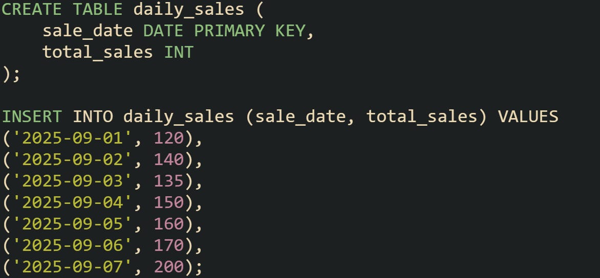
If you calculate the 7-day average on September 7, the result is (120+140+135+150+160+170+200)/7, which comes out to about 153.57. That value smooths the ups and downs across the week into a single figure.
Smaller windows like 3-day averages react faster to changes but can look jumpy. Larger windows like 30-day averages react slower but make trends more stable. Choosing seven days gives a balance that many domains, from finance to epidemiology, find useful.
Why SQL Handles This Well
Relational databases are designed to operate across sets of rows. Aggregate functions such as AVG() collapse a group into one number, but window functions go further by letting you keep each row while still calculating aggregates across a moving frame. That’s what makes them perfect for rolling averages.
Take this example that doesn’t yet involve rolling, just a group average.

That gives one number across the whole table. Useful, but it hides the trend over time.
Now compare it with a window function that attaches the average to each row while still keeping the detail.
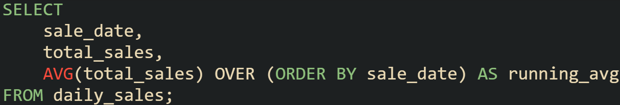
This form produces a running average from the start through each row. You can see how SQL attaches aggregates without collapsing rows away.
The reason SQL is good at this lies in its logical evaluation order: window functions run after FROM, WHERE, GROUP BY, and HAVING, and before the outer SELECT DISTINCT, ORDER BY, and LIMIT. That lets the database keep a moving frame in memory and update the calculation as it goes, rather than recomputing the whole frame from scratch each time.
Window Frame Mechanics
Window frames define how far backward and forward the function looks relative to the current row. For a rolling 7-day average, you want six preceding rows plus the current row. The SQL syntax makes that explicit.
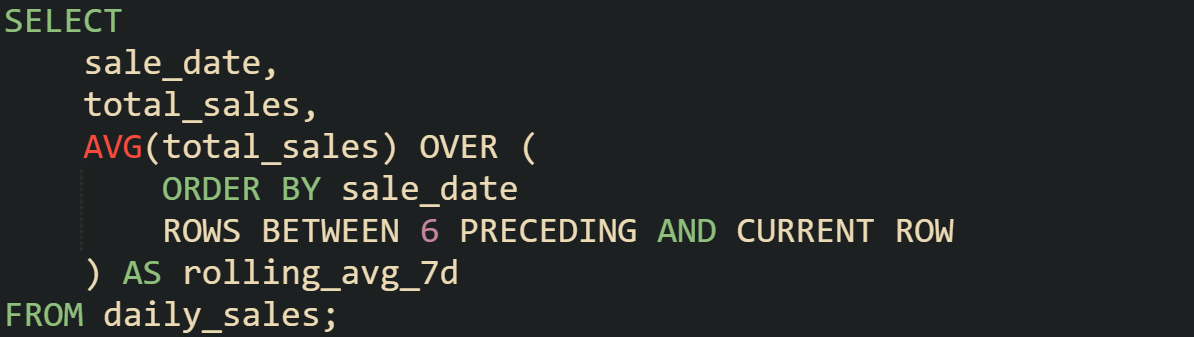
That clause says: order rows by date, then for each row, look at the current one plus six before it. The frame shifts as the database moves row by row.
Something worth knowing is how the boundaries change. On the first day, there aren’t six rows behind, so the average uses only the rows that exist. The second day has two rows, the third has three, and so on until the seventh day when the frame is full. After that, each new row pushes out the oldest value and brings in the newest one.
Window frames aren’t limited to numeric counts of rows. Some databases allow interval-based frames where you can say “look back 7 days” instead of “look back 6 rows.” That option becomes useful when your dataset has missing days or irregular intervals, though not every engine supports it in the same way.
Writing Queries for a Rolling 7 Day Average
Rolling averages become useful only when you can express them in a way the database understands. SQL provides the tools to define order, calculate aggregates, and handle gaps, but the design of the query changes depending on the situation. A well-built query balances accuracy with performance while keeping the results easy to interpret.
Sample Data Setup
Practical work always begins with a dataset. Suppose you’re working with a simple table that tracks daily visitors to a website.
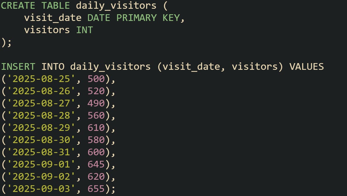
With a table like this, you have a steady stream of data points ordered by date. That order is the foundation for every rolling average, because without a defined sequence the database can’t know how to build a moving frame.
It’s worth checking that your column type for the date is consistent. Using a text column that looks like a date won’t sort correctly. An actual DATE or TIMESTAMP type guarantees the right order.
Using ROWS BETWEEN
The most common way to create a rolling average is with AVG() applied over a window of rows.
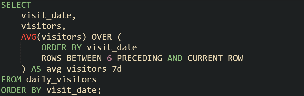
This query defines a frame of seven rows, moving forward one row at a time. The average gets recalculated on each step, and the result is attached to that specific row.
To make the mechanics easier to grasp, you can run the same query with a smaller frame.
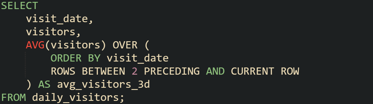
Looking at both results side by side helps show how the size of the frame changes the smoothness of the trend. The smaller frame reacts faster but looks noisier. The 7-day version settles those fluctuations and brings longer movements into focus.
Differences Between ROWS and RANGE
Window functions allow more than one way to define a frame. The two most common are ROWS and RANGE. They look similar but behave differently once you put them to work.
ROWS counts the exact number of physical rows in the order defined. That’s why ROWS BETWEEN 6 PRECEDING AND CURRENT ROW always includes seven rows when they’re available.
RANGE frames by the value in the ORDER BY, not by a row count. With dates or timestamps, a clause like RANGE BETWEEN INTERVAL '6 days' PRECEDING AND CURRENT ROW includes every row whose ordering value falls in that 6-day span, plus any peers with the same current value.
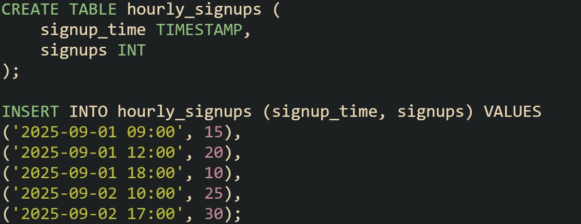
To see the difference, start with a table that allows duplicates for the same day.
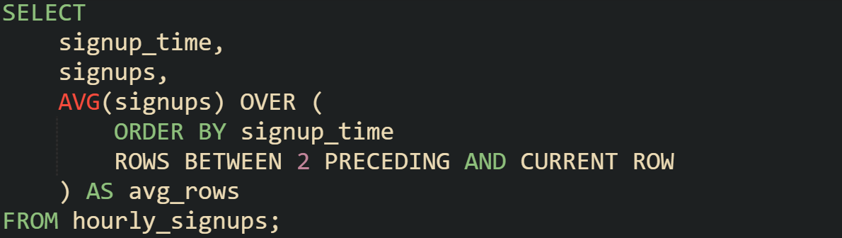
A query using ROWS treats each record separately.
Switching to RANGE changes the frame to cover a span of time, not a count of rows.
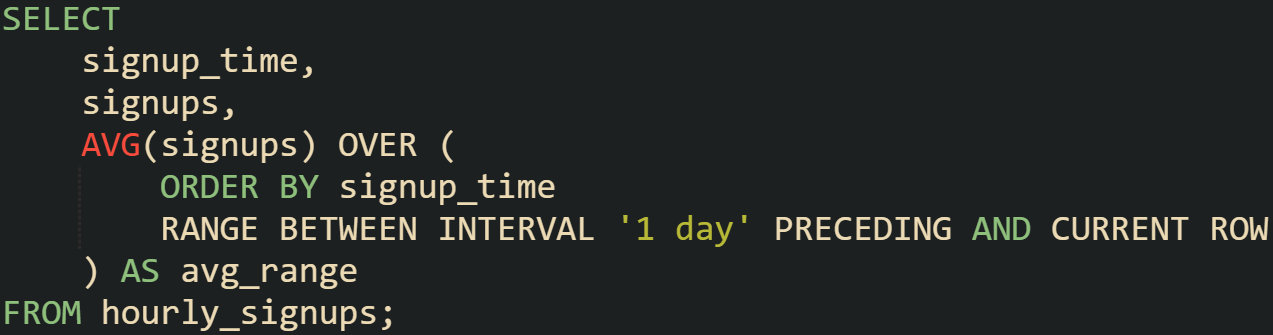
This difference matters when you’re dealing with irregular intervals or repeated timestamps. For a steady daily table, ROWS is often the safer choice, but when timestamps repeat or have uneven gaps, RANGE can make more sense.
Handling Missing Days
Real-world data often has gaps. If you’re averaging over calendar days, those gaps can skew results because the database only counts rows that exist. Filling in missing dates makes the rolling frame accurate.
In PostgreSQL, a common way to solve this is by generating a calendar of dates and joining it to the main table.
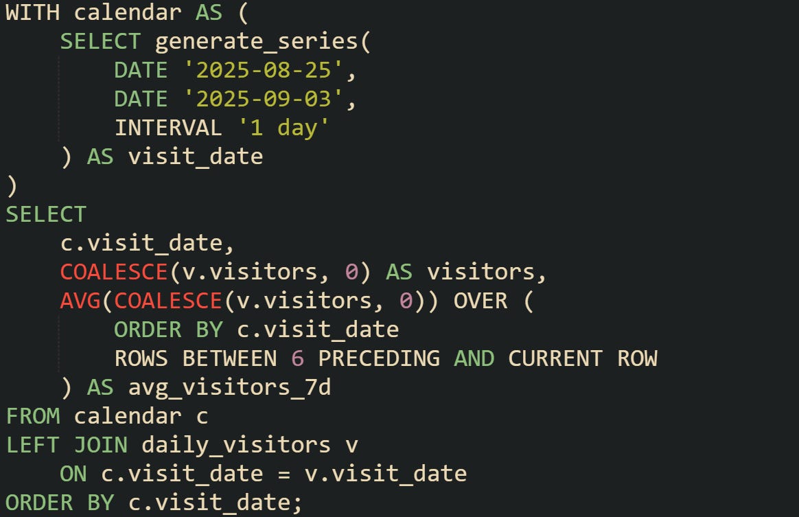
This guarantees that the frame always spans seven consecutive days. If a date has no data, it still counts in the timeline with a placeholder value.
For databases that don’t have generate_series, you can create a separate calendar table ahead of time and reuse it. That table acts as a backbone for every time-based report.
Performance Considerations
Window functions can handle millions of rows, but performance depends on how you prepare the data. Ordering is required for rolling averages, so indexing the date column is critical. That index lets the database retrieve rows in the right order without scanning the entire table each time.
On very large datasets, partitioning can help. If you partition your data by year or month, queries that focus on a smaller slice won’t force the engine to scan the entire table. Some databases also use parallel execution plans that distribute window calculations across multiple workers.
Different systems have their own quirks. MySQL only gained full support for window functions in version 8.0. SQL Server and Oracle have mature implementations, while PostgreSQL has strong support for both ROWS and RANGE. It’s worth knowing what your environment supports so you can pick the right syntax without surprises.
Practical Use Cases
Rolling averages appear in many fields because they smooth short-term noise into something more readable. A weekly view of user logins shows whether engagement is trending up or down without being distracted by day-to-day fluctuations. In finance, rolling averages track moving prices and smooth out volatility. In public health, rolling averages are used to report case counts in a way that avoids confusion from daily swings.
Here’s a query that applies the same technique to a dataset of daily revenue.
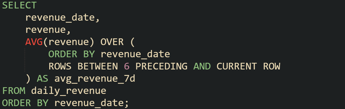
That pattern works across almost any numeric measure tied to a timeline. Whether it’s sales, signups, or sensor readings, the database is applying the same mechanics: take the current row, look back six more, average the values, and attach the result without losing the row detail.
Conclusion
A rolling 7-day average works because the database holds a moving frame of rows, recalculates the mean at every step, and attaches that number back to each row without discarding the detail. Window functions make this possible through their ability to look backward across a defined range, update the frame as new rows arrive, and keep the calculation consistent throughout the timeline. When you write a query with AVG() and a frame defined with ROWS BETWEEN, you’re telling the engine exactly how to move across the data. That simple mechanism is what turns a string of daily values into a smoother curve that reveals longer movements in a dataset.
