

Finding the most recent row for each group in a dataset is a common task in data work. It’s often needed when you want the last login date for every user, the most recent order for each customer, or the newest update for a project. While the idea is simple, how the database processes the query can make a big difference in performance, especially with larger datasets. Two well-supported ways to get this done are with ROW_NUMBER() in window functions or with correlated subqueries.
Both produce the same final output, but the way they operate behind the scenes is not the same. Learning how each method works makes it easier to choose the one that best fits your database system and the size of your data.
Using Window Functions with ROW_NUMBER
Window functions give you a way to work with related rows while still keeping all the original detail. They process after filtering and joins, so you can create values based on other rows without losing them from the result set. ROW_NUMBER() is one of the most practical of these functions, assigning a sequence number to rows in a defined group and order. After that numbering is done, it becomes simple to keep only the first row from each group. This method is supported in current releases across major engines: PostgreSQL 8.4+, SQL Server 2005+, Oracle 8i+, SQLite 3.25+, MySQL 8.0+, and MariaDB 10.2. It also keeps the SQL readable and easy to adjust if the grouping or sort order changes later.
How the Database Processes ROW_NUMBER
When you write a query with ROW_NUMBER() and a PARTITION BY clause, the database first groups the rows based on your partition column. Within each group, it sorts them according to your ORDER BY rule so that the most relevant row appears first. That sorting can be ascending or descending depending on whether you need the earliest or the latest record. After the sort step, ROW_NUMBER() assigns a number starting at one and increases it for each row in the group. This numbering is computed during SELECT evaluation after rows are filtered and joined. The engine may sort or buffer data to do it, so no self-join is required to pick the top row. The last step is filtering for the number one row in every group, which is typically done in an outer query.
Here’s a simple example with a table that tracks page visits:
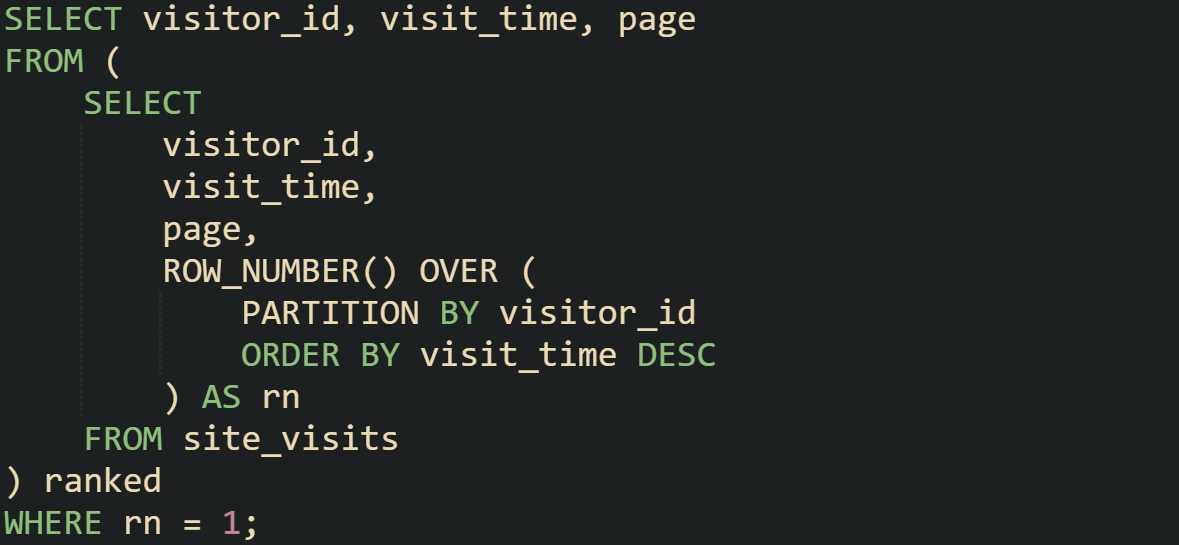
PARTITION BY visitor_id restarts the numbering for each visitor, while ORDER BY visit_time DESC makes sure the most recent visit gets the first number.
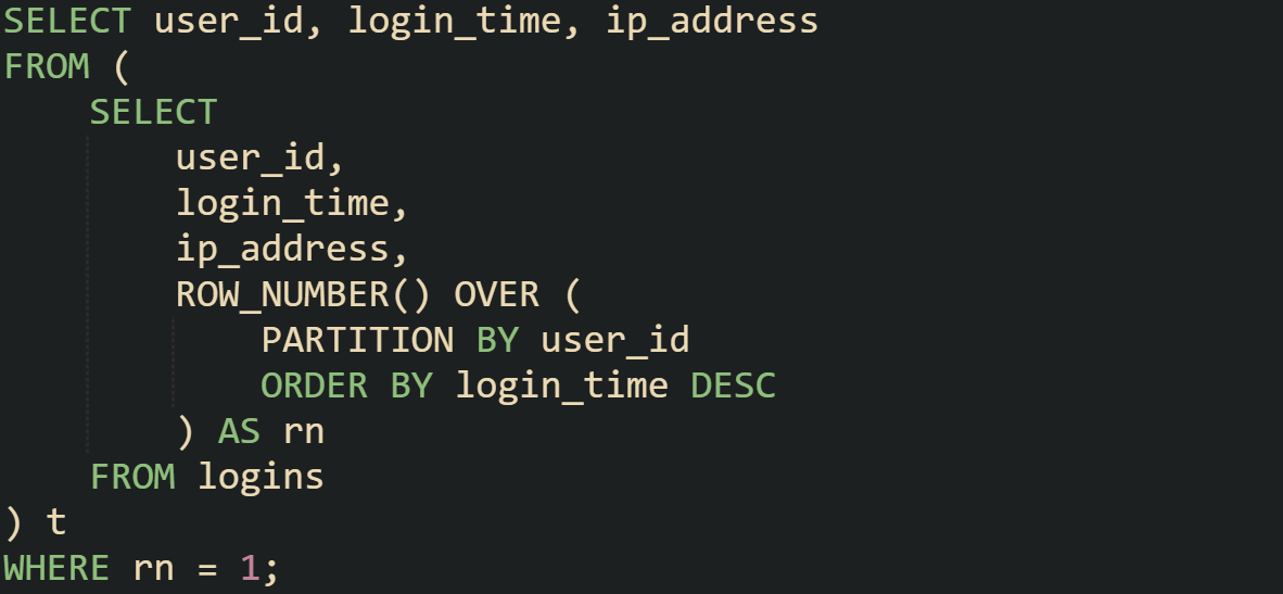
Example with Latest Login per User
A login table is a common place where you’ll want the most recent record per user. ROW_NUMBER() makes this direct and avoids extra joins:
This structure can be adapted to more specific needs. Suppose you want the latest login for each user but only from a particular location. You can apply that filter before numbering, which reduces the amount of data processed in the window function:
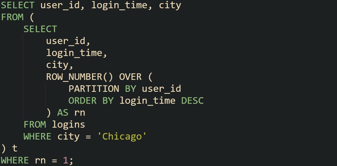
Filtering inside the subquery makes sure that the numbering step only works on relevant rows, which can improve performance in large datasets.
Optimizing This Method in Practice
When a query partitions by a column and sorts by another, matching that combination in an index can help the database skip unnecessary work. For example, if the partition column is user_id and the ordering column is login_time, an index on (user_id, login_time) can allow direct access to the top rows. Without that match, the system may have to sort data for each group in memory, which grows slower with bigger tables.
With a ROW_NUMBER() filter like WHERE rn = 1, most engines still evaluate the partition and its sort. A composite index on (partition_key, order_key) reduces sorting work. PostgreSQL, SQL Server, and MySQL evaluate the window after the input is ordered by the partition and order keys. In MySQL 8.0, filtering on rn = 1 still computes the window for each partition, the optimizer can reuse ordering across compatible windows, but it does not stop early per partition. The difference is most noticeable with large datasets where groups have many rows.
Correlated Subqueries
A correlated subquery works by running a smaller query for every row the main query reads. While this might sound like it would always be slower, modern database optimizers often handle it efficiently, especially when the right indexes are present. For the problem of finding the latest record per group, the subquery’s job is usually to identify the maximum date or timestamp for that group, and the main query then checks whether the current row matches that maximum value.
The beauty of this method is its simplicity in terms of SQL structure. You don’t need to learn advanced functions, and it works in nearly every database version still in active use. That makes it an excellent choice in systems where window functions aren’t available.
How the Database Processes a Correlated Subquery
When a correlated subquery runs, the database starts with a row from the main query, passes its grouping value to the subquery, and executes that inner query to produce a result specific to that group. In the case of getting the latest record, the subquery finds the maximum timestamp for the matching group. The main query compares the current row’s timestamp with that maximum and decides if it should be part of the output.
While the concept is row-by-row execution, many database engines avoid physically running the subquery in a loop by reusing cached results or transforming the logic into an indexed lookup. This means that performance can be much better than the logical description suggests, but only if the indexing matches the query pattern.
Here’s a simple example for a table of product updates:
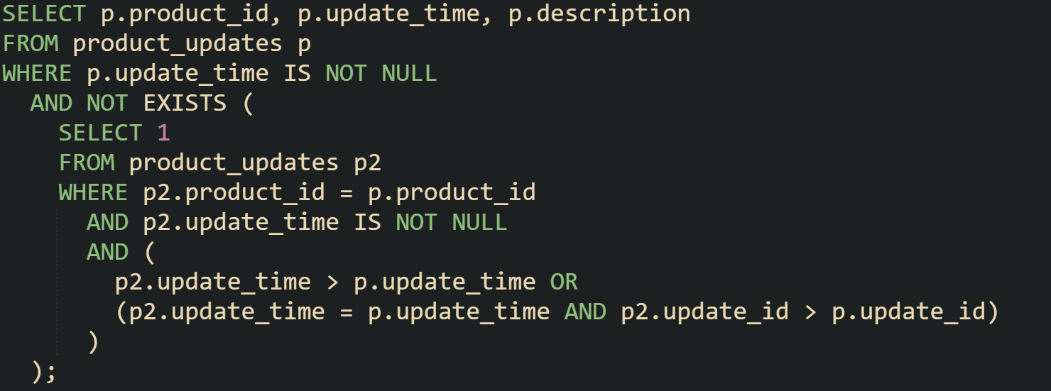
The inner query checks for any row with the same product_id that has a later update_time or the same update_time with a higher update_id. If it finds one, the current row is dropped. Rows that have no later match stay in the results, and any with NULL timestamps are skipped.
Most Recent Order per Customer Example
In an orders table, you might want the most recent order for each customer. A correlated subquery can handle this with a single filter in the main query:
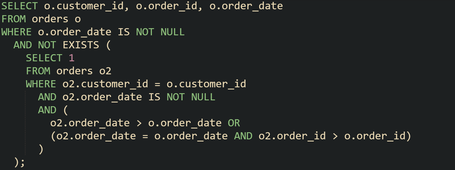
A row only stays in the results when there’s no other order from the same customer with a later order_date. If there’s a tie on order_date, the one with the higher order_id is treated as later and removes the current row from the results. This tie-breaker makes sure that only one row is kept for each customer, even when two orders share the same date. Any row where order_date is NULL is excluded, so the output only contains orders with a valid timestamp to compare.
You can expand this pattern for other constraints. Suppose you only want the latest completed order for each customer, not pending ones:
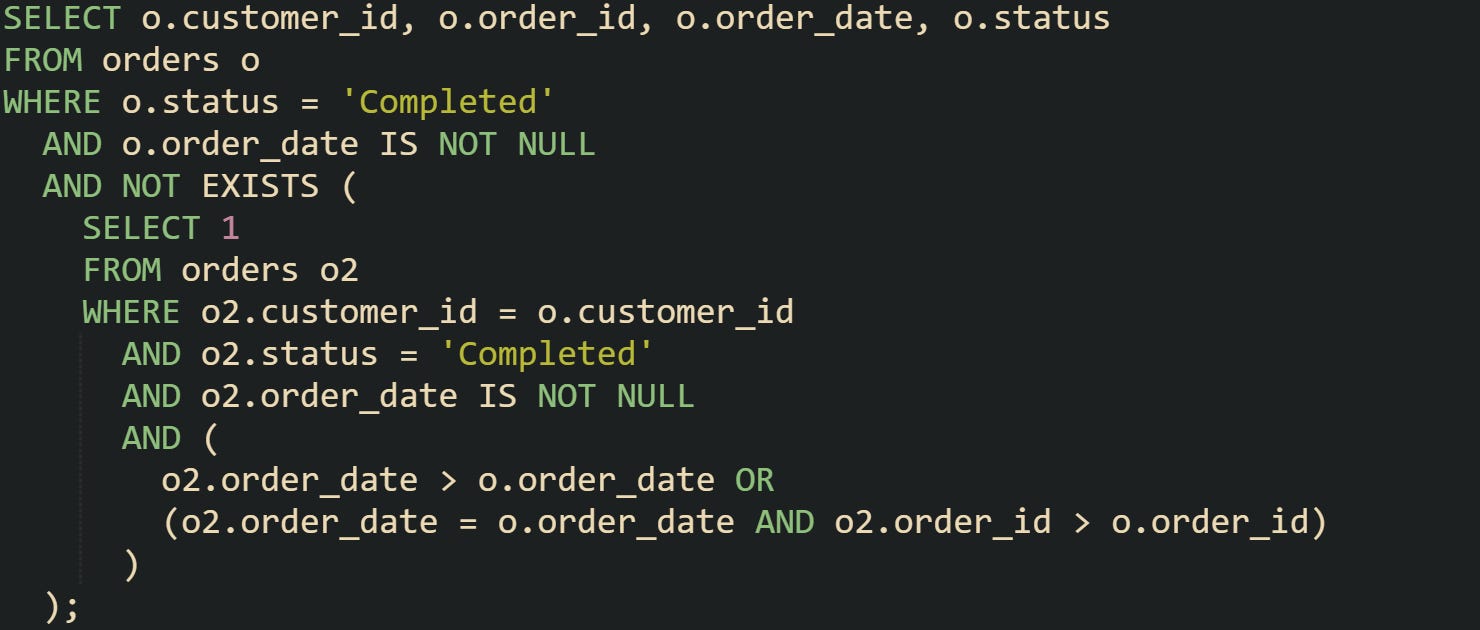
The condition in the inner query keeps the comparison focused entirely on orders marked as completed. That means pending or canceled orders won’t affect which row is kept as the latest. Within those completed orders, the same date and ID logic applies, so a row is removed if there’s another completed order with a later order_date or the same date but a higher order_id. Any rows with NULL dates are ignored, so incomplete or invalid date values don’t interfere with the comparison.
Making This Pattern Run Faster
Accurate table statistics help the planner estimate group sizes and choose index seeks or sorts that keep this pattern fast. If estimates drift, you can see slower scans even with a composite index in place. Modern database engines can also transform the logic of this type of query before running it. In some cases, the optimizer turns the subquery into an index seek, which can make it much faster than the basic description suggests. This tends to work well when table statistics are accurate and the values in the grouping column are spread evenly.
When there’s no suitable index or when data distribution leads to less effective lookups, the database may need to calculate the aggregate for every group through a wider scan. That extra work can add noticeable time as the table grows, making indexing choices and statistics maintenance more important for keeping the query efficient.
Conclusion
Getting the latest record for each group comes down to how the database organizes and compares data during the query. With ROW_NUMBER(), the work is handled in one pass after grouping and sorting, which makes it easy to trim the results to just the top row. A correlated subquery takes a different path, checking each row against the maximum value for its group and keeping only the matches. Both depend heavily on indexes to avoid extra scans and sorts, and both can benefit from how the query planner chooses to run them. Having a clear picture of how each method moves through the data makes it easier to match the technique to the database and workload you have.
