

Parent child data shows up in many systems. Product categories, comment threads, organizational charts, and menu trees all follow the same idea. One row points to another row as its parent, and many queries need both in a single result set. SQL gives you several ways to handle this. Careful joins can pull parent and child rows side by side, and common table expressions can walk deeper trees so nested data flattens into a form that is easy to read and process.
Parent Child Table Relationships
Generally speaking, parent child tables give structure to data that falls into levels, such as a top row that owns several related rows underneath it. Product catalogs, threaded comments, and staff charts all rely on this idea. Foreign keys carry that structure inside the database so queries can move from one level to another without extra storage or duplicated values.
How Parent Child Tables Are Structured
Relational tables usually represent a parent link with a foreign key column on the child side. That column stores the primary key of the parent row, so one parent can have many children while a child points to only one parent within that relationship. Many schemas separate parent and child into different tables when they carry different attributes. Departments and employees fit that shape. Departments hold information such as a name and a cost center code, while employees store personal data and a reference to the department they belong to.
 NOT NULL, cost_center VARCHAR(50) NOT NULL, active BOOLEAN NOT NULL DEFAULT TRUE ); CREATE TABLE employee ( id BIGINT PRIMARY KEY, full_name VARCHAR(200) NOT NULL, department_id BIGINT NOT NULL, hire_date DATE NOT NULL, CONSTRAINT fk_employee_department FOREIGN KEY (department_id) REFERENCES department(id) );")
Foreign key fk_employee_department tells the database that employee.department_id must match an existing department.id. Indexes on these columns let joins move quickly between departments and employees when queries connect the tables.
Self referencing trees keep parent and child rows in one table. Category hierarchies in a shop or content management system fall into this group. Top level categories have no parent, while lower level categories point back to other rows in the same table.
 NOT NULL, parent_id BIGINT NULL, slug VARCHAR(200) UNIQUE, sort_order INT NOT NULL DEFAULT 0, CONSTRAINT fk_category_parent FOREIGN KEY (parent_id) REFERENCES category(id) );")
Root categories store parent_id as null, and subcategories store the id of their parent row. Column sort_order lets queries put siblings in a stable sequence under the same parent, while slug provides a stable identifier for URLs or external references. Indexes on id, parent_id, and sometimes sort_order support common lookups such as finding all children under a parent or ordering those children for display.
Many self referencing tables add flags such as active or visible so queries can skip retired parts of the tree while keeping links intact. That keeps the structure stable while allowing soft deletes or archival behavior without breaking foreign key rules.
How One Query Can Return Parent Child Rows
Many queries need both parent information and child information at the same time. A staff list that shows employee names and department names, or a product grid that shows category names next to products, both rely on data from two levels returning in a single result set.
Joins supply that link inside a single statement. The join condition matches a foreign key on the child table to a primary key on the parent table. That condition tells the database which rows belong together when it scans or probes indexes.

This query returns one row per employee, with department attributes present on the same line as employee attributes. Sorting by department name, then by employee name, keeps related rows close together near the top or bottom of the result.
Self referencing tables rely on a similar idea but use aliases so the same table can appear on both sides of a join. One alias represents the parent side and the other alias represents the child side. That structure lets queries show a child category next to the category that owns it while still reading from a single physical table.
Lots of applications then pass this flattened result set to a user interface or reporting layer that groups rows by parent id. The raw SQL already carries all details in one batch, so later steps can reshape the result into trees, lists, or grids without running more database calls.
How Joins Match Parent And Child Rows
Joins match parent and child rows through equality tests between columns. Parent tables supply a primary key column, while child tables supply a foreign key column. Conditions such as e.department_id = d.id guide the engine as it walks indexes or scans table pages.
Inner joins keep only rows that have a match on both sides. When a child refers to a parent through a foreign key and both rows exist, an inner join returns that pair. Missing parents or children do not appear in the result.

Every row from this statement represents a valid employee and a valid department. Foreign key constraints normally prevent an employee from pointing at a missing department, so inner joins on well enforced parent child relationships tend to reflect that integrity.
Left joins keep all rows from the table on the left side of the join, even when no matching row exists on the right side. Parent child queries that need parents with zero children rely on this form. A department without employees still appears, with child columns set to null.

Departments that currently have no employees show a null employee id and name. That behavior makes it easy to see gaps or new departments that have not yet hired anyone, while departments with existing staff produce multiple rows.
Self joins extend this idea by treating the same table under different aliases. A query can join categories to their parents with one join, then join the parents to grandparents with another. That technique handles a fixed depth of hierarchy, such as three levels of navigation, by chaining joins layer by layer. Join order inside the FROM clause does not force the engine to read tables in that exact sequence. Planners can rearrange inner joins while keeping the same logical result, often choosing the smallest or most selective tables first. Foreign key relationships and index statistics guide those decisions so that parent child joins scale as data volumes rise.
How A Single Query Can Filter Parents And Children
Parent child queries almost always include conditions that restrict rows. Filters may target status flags, date ranges, tenant identifiers, or names. A single statement can filter parent rows, child rows, or both, and the placement of those filters affects which combinations stay in the result.
Filters in a WHERE clause apply after the join logic has created joined rows. Conditions there see parent and child columns at the same time. When both sides must meet a rule, WHERE is the natural home for that condition.

Result rows from this query always come from active departments. Employees may be null where a department has no staff yet, because the filter does not require a matching employee. Only the parent status flag matters for row survival.
Filters attached directly to a join condition behave in a different way. Conditions written in the ON clause limit which rows count as matches for that join, without automatically removing the row from the outer query. Parent rows from a left join remain, while child columns become null if no children satisfy the join conditions.
Let’s consider a case where new hires need to be highlighted for reporting while older hires are still stored in the table. A query can treat recent hires as matches and older hires as non matches without losing any departments.

Every active department appears in the result. Rows where no employee satisfies the hire date condition show nulls in the recent employee columns. That behavior arises from the filter placement, because the hire date check lives inside the join and not in the WHERE clause.
Self referencing hierarchies use the same principles. Filters applied in the join condition can restrict which child categories count as matches, such as categories marked visible, while filters in the WHERE clause can restrict which parent nodes show up at all. Through careful placement of conditions, a single query can express rules about visibility, status, and time ranges for both parents and children without splitting work across multiple statements.
Query Patterns For Parent Child Lookups
Parent child tables support several query forms, and each one fits a different kind of question. Some queries only care about a parent with one layer of children, others have to walk deeper hierarchies, and many reports need both detailed rows and summary numbers in the same result set. Keeping these lookups inside a single statement helps keep filters, joins, and sorting rules all in one place, while still giving application code a flat result that is easy to work with.
Single Level Lookups With Joins
Many systems store relationships that stop at one parent level, such as a blog post with comments, an order with line items, or a customer with invoices. Queries in that category usually only need parent and child rows side by side, with no need to walk further up or down any tree.
Joins give a direct path from parent to child in one statement. An order with its line items is a common case. Orders live in one table, items live in another, and a foreign key points from line items to the owning order. A query that lists all items on recent orders, along with order level attributes, can look like this:
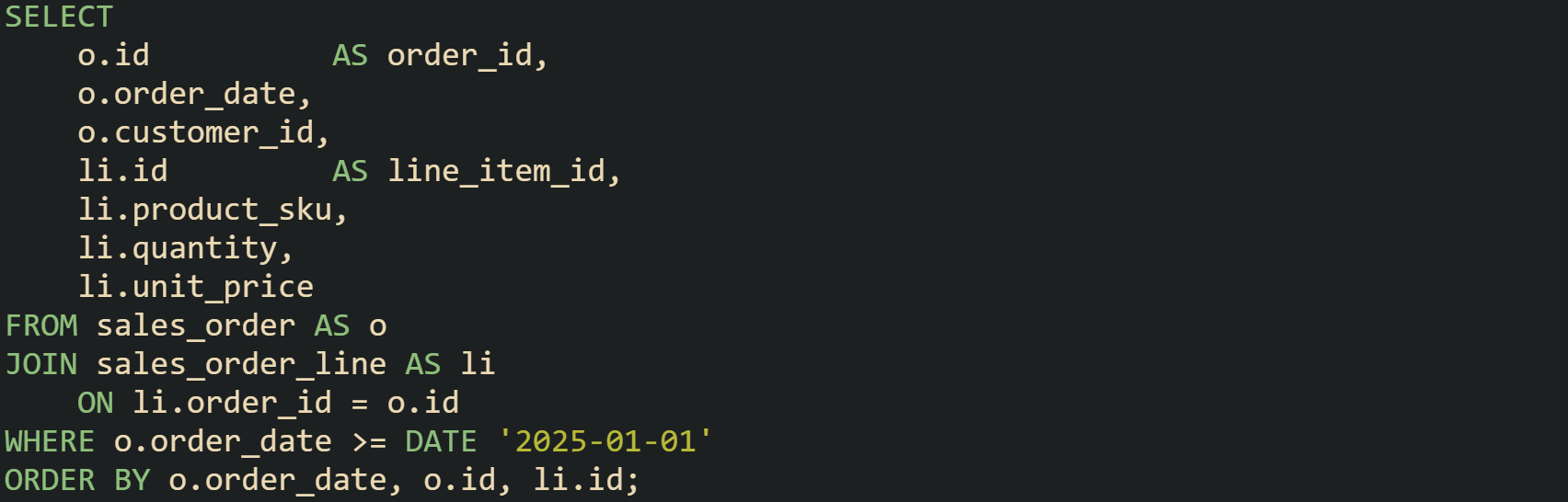
Result rows from that statement carry both order data and line item data. Many user interfaces can render grids or tables straight from this kind of output without more joins in application code.
Direction of the join in the text does not change which rows match. A query that begins with the child table and joins back to the parent uses the same condition in reverse. That shape can work better when filters sit on the child table, because the planner can start from the most selective side and then visit parents.

This query begins from line items that carry a specific product code, then chains back to the order level data so that the final result still carries both layers.
Single level parent child data sometimes needs a choice between inner and outer joins. Inner joins keep only pairs where both parent and child exist. Outer joins start from one side, usually the parent, and preserve those rows even when no child matches. Catalogs where every product must have a valid category fit inner joins. Department tables that include new departments without any staff yet fit left joins, so departments still appear with null child columns until hiring catches up.
Self joins support single level lookups when parent and child rows sit in the same table but the query only needs a direct parent link and not a full tree. Menu structures where items can have one parent item but never go deeper than two levels can stay with a self join and skip recursive logic. That keeps SQL readable while still letting the database enforce foreign keys and support future growth when additional query styles appear.
Hierarchies With Recursive CTEs
Some data grows beyond a single level. Category trees, file system folders, corporate reporting lines, and menu structures can all have many layers from root to leaf. Joins can handle one or two layers with chained self joins, yet that technique turns awkward once the maximum depth is unknown or large. Recursive common table expressions give SQL a way to keep the logic in one block while the engine handles as many levels as exist in the data. Recursive CTEs have two parts inside the same WITH definition. The first part, sometimes called the anchor, selects starting rows such as roots. The second part refers back to the CTE name and pulls in children of any rows already collected. Folder trees give a good example:
) AS full_path FROM folder WHERE parent_id IS NULL UNION ALL SELECT f.id, f.name, f.parent_id, ft.depth + 1 AS depth, CONCAT(ft.full_path, '/', f.name) AS full_path FROM folder AS f JOIN folder_tree AS ft ON f.parent_id = ft.id ) SELECT id, name, parent_id, depth, full_path FROM folder_tree ORDER BY full_path;")
Execution starts from folders that have no parent, treats those as depth zero, then repeatedly joins back to folder to find children. Every loop through the recursive part increments the depth and extends full_path, so the final result tells both where a folder sits and how deep it is.
Many hierarchies need a way to focus on one branch instead of the entire tree. A query that starts from a chosen node in the anchor part of the CTE gets that result. Suppose administrators want to list only the subtree under a folder named reports:
 SELECT id, name, parent_id, depth FROM folder_subtree ORDER BY depth, name;")
This time the anchor pulls only the reports folder, and the recursive join walks down from that point to collect children, grandchildren, and so on. Results carry depth, which makes it easier for a rendering layer to indent rows or apply different formatting for roots and leaves.
SQL standards define SEARCH and CYCLE clauses that sit with recursive CTEs in some engines. SEARCH can add ordering columns that describe a traversal order such as breadth first or depth first. CYCLE helps detect loops in faulty data, such as a folder that points to itself or two folders that refer to each other as parent and child. Some database engines offer support for these clauses, which gives extra control for advanced tree operations beyond basic hierarchy flattening.
Indexes on id and parent_id columns still matter in recursive queries. Each recursive step needs to find children for a set of parent ids, so lookups on parent_id should rely on an index rather than full table scans. Large hierarchies can benefit from filtering in the recursive part as well, such as stopping at a certain depth or excluding inactive nodes, which keeps the working set from growing without limit during recursion.
Parent Child Lookups With Aggregates
Many questions about parent child data mix detailed rows with summary numbers. Reports on customers and their orders, articles and their comments, or projects and their tasks frequently want totals per parent and also need to see the individual children that make up those totals. SQL can combine aggregates and joins so that both views appear in one result.
One common form collects summary data in a CTE and then joins that CTE to detailed child rows. A sales report that needs order totals per customer while still listing every order fits well here:
 AS order_count, SUM(total_amount) AS total_spent FROM sales_order GROUP BY customer_id ) SELECT c.id AS customer_id, c.email, tot.order_count, tot.total_spent, o.id AS order_id, o.order_date, o.total_amount FROM customer AS c LEFT JOIN customer_order_totals AS tot ON tot.customer_id = c.id LEFT JOIN sales_order AS o ON o.customer_id = c.id ORDER BY CASE WHEN tot.total_spent IS NULL THEN 1 ELSE 0 END, tot.total_spent DESC, o.order_date DESC;")
The CTE runs first and leaves one row per customer in customer_order_totals, holding only aggregated numbers. The main query then attaches those totals and detailed orders to every customer row. Customers with no orders appear with null totals and no matching orders, which can help highlight inactive accounts.
Window functions give another tool for this space and can remove the need for a separate CTE in many cases. Aggregates such as COUNT, SUM, and AVG can operate over partitions, where each partition groups rows that share parent attributes. This category and product example makes that make more sense:
 OVER (PARTITION BY c.id) AS product_count_in_category FROM product AS p JOIN category AS c ON p.category_id = c.id ORDER BY c.name, p.name;")
Every product row carries the count of products in its category through the window function COUNT(*) OVER (PARTITION BY c.id). Grouping happens logically in the window function while the underlying rows remain separate, which means aggregates and detailed data share a single pass over the joined result.
Window functions cover more than just COUNT. Queries can attach maximum or minimum child values per parent, such as the most recent comment date per article or the largest invoice total per customer, while still keeping one row per child. That flexibility helps when reports need both per parent statistics and row level inspection without multiple statements. Aggregates also appear directly on parent child joins with GROUP BY at the end of the query. Reports that list only parents with no detailed child rows, such as departments with employee counts but no employee lines, can group on parent columns without a CTE or window function, which suits dashboards and other high level summaries, while CTE and window function forms handle combined detail and summary in one result.
Conclusion
Parent child queries in SQL rest on how tables link through foreign keys, how joins pull related rows into one stream, and how CTEs or window functions stack on top of that base. Strong habits around modeling parents and children, writing precise join conditions, and choosing between inner, outer, and recursive forms give you enough control to flatten hierarchies into results that match what calling code expects without extra passes through the data.
