

Turning Rows Into Columns To Build Pivot Tables In SQL
Build pivot-style outputs using pure SQL


When you need to build a report from relational data, the default layout isn’t always what works best. Sometimes the data you have is stored in rows, but what you really need is to turn values from one column into headers so each category gets its own column instead. This is called pivoting the data. Most engines use conditional aggregation for this. Some, like SQL Server and Oracle, support a PIVOT clause directly. Either way, you can reshape the result using a simple combination of CASE expressions inside a GROUP BY.
How Row Data Is Transformed Into Columns
When a report needs numbers arranged by category across the top, but your data is stored with values running vertically down a single column, you’re working against the grain of how relational tables are structured. Most SQL databases store rows in a flat format, which works well for inserts and updates but isn’t always how people want to read data. If you’ve been asked to put categories into columns, what they want is a pivot table layout. SQL doesn’t automatically do this for you, but there’s a reliable way to reshape the output using conditional logic inside grouped queries. Each output column comes from a clear condition written in a CASE expression, evaluated during aggregation.
Row-Based Format And What We Want Instead
Let’s say there’s a table called monthly_sales that tracks sales totals by region and product. It might look like this:

Each row is one combination of region and product, which is tidy for storage but less useful for reports that compare product totals side-by-side. The goal is to shape the output into this format instead:

The header now has product types across the top, and the totals fill in based on region and product matches. This isn’t automatic. You have to tell SQL exactly how to assign values from one column into new columns, and that’s where conditional aggregation comes in.
Using CASE With Aggregation
The technique that drives this is built on combining CASE expressions with aggregation functions like SUM. You write one expression for each column you want to show. Each expression uses CASE to look at the product type and either return the value or return zero, depending on whether it matches.
Here’s the basic pattern:

This says, “only include the value in the sum if the product is Laptop, otherwise treat it as zero.” That logic runs inside each group defined by GROUP BY.
Let’s look at the full query that turns the original rows into the new layout:
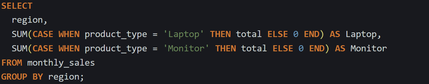
Here’s what happens as the query runs:
The database finds all the unique values in the
regioncolumn.It groups the rows by each region.
Inside each group, it processes the
SUM(CASE...)logic for Laptop and for Monitor.
Each column is driven by one condition. If a region doesn’t have a row for a certain product type, then all the CASE checks for that product will return zero, and the total ends up being zero. You could leave out the ELSE 0 part, but that would result in NULL values instead of zeros, which can be messy in reports.
Each column in the output is built manually, and each one has its own filter condition hardcoded. This is the tradeoff: you get precision and full control, but it takes work.
How The Query Engine Handles It
The SQL engine still treats this like any other grouped query. There’s nothing special about the pivoted shape in terms of what the engine sees. It runs a GROUP BY, processes each row one at a time, and evaluates each CASE expression inside the aggregate functions.
Think of it as filtering on the fly. Each time the engine hits a row, it checks the CASE to see whether to use the value or not. If the condition is true, it includes the value in the sum. If not, it skips it or returns a placeholder like zero. These are not computed later and are resolved during the aggregation step, while the group is being built. Internally, the SUM(CASE...) structure becomes part of the aggregation plan. It’s no different from doing a sum on a column, except you’ve told SQL to only include some of the values. Every time SQL sees one of these aggregates, it needs to evaluate the logic across each group it builds.
Because you wrote the logic yourself, SQL doesn’t try to generalize it. It evaluates exactly what you wrote, using the condition to split the values into separate columns. There’s no guesswork or dynamic mapping. You’ve told it, “only show this value when the product type matches this label,” and SQL does exactly that. This is why pivoting works so predictably. You’re not asking the database to figure anything out on its own. The structure of the query lays out the rules clearly, and the engine just runs them as part of the standard grouping and aggregate process.
Expanding To More Columns
Once you’ve written one or two of these, adding more is just more of the same structure. If your data includes other product types, you need to write an expression for each one.
For example, if the data has a third product type called Keyboard, just add one more line to the query:
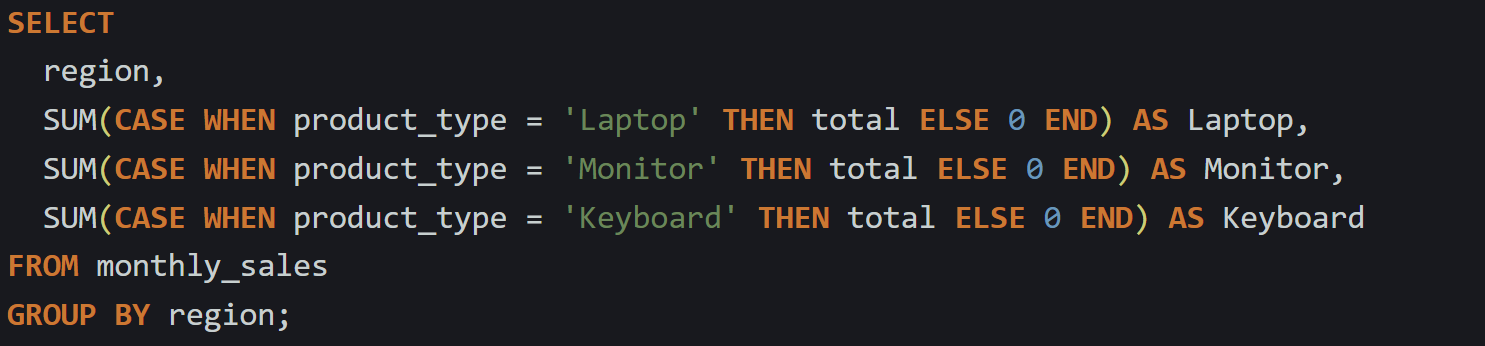
The process stays the same. SQL groups by region, then evaluates each of those conditional sums one by one. There’s no technical limit on how many columns you can generate this way, but if the list of product types is long or changes frequently, you’ll need to manage the list elsewhere, maybe by generating the query dynamically or filtering to just a subset. That’s a separate concern from the mechanics, which stay the same regardless of how many expressions you include.
One helpful pattern is to use aliases that match the product type names exactly, so the output looks natural and matches what people expect to see in a report. As long as the product types are known ahead of time, this method gives you a repeatable way to control exactly what shows up in your result. You’re reshaping a flat row structure into a cross-tabbed layout, column by column, using nothing more than conditions and grouping. There’s no need to restructure the database or store the data differently. You’re just shaping the query to produce a different view.
Variants And Behavior In Different Scenarios
The general pattern for pivoting with CASE and GROUP BY stays the same no matter the dataset, but how the output behaves depends on the data itself. Different edge cases can change how the numbers show up, especially when certain values are missing, when you're tracking more than one field, or when column names affect how reports are read. It helps to understand how these details behave so the output comes out clean and predictable.
When Values Are Null Or Missing
Sometimes, you’ll run the query and see that some cells are empty. This usually happens when a group doesn’t have any matching rows for a specific product, status, or category. The engine doesn’t raise an error or skip the group. Instead, it runs the logic, but the CASE conditions never pass, so nothing gets added up.
By default, if you don’t include an ELSE clause in your CASE, SQL returns NULL for rows that don’t match the condition. Here’s how that looks:
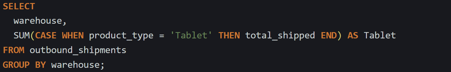
If a warehouse didn’t ship any Tablets at all, the sum expression has no value to add. Without an ELSE, the return becomes NULL, which can throw off exports or reports that expect to see zero.
Adding ELSE 0 fills those blank spots with a numeric zero:

This version makes sure every group produces a number, even if there were no matching rows. That’s usually what you want when pivoting, so the layout stays consistent.
Also, if your source data already contains nulls in the column you’re aggregating, those are ignored by SUM and AVG unless you account for them first. It’s usually fine, but if totals don’t look right, it’s worth checking whether the total_shipped or other metric column has any missing values.
When There Are Multiple Metrics
A pivot doesn’t need to stop at one field. You can pull in other metrics by repeating the same pattern for each one. This is useful when the report needs totals and counts, or maybe revenue and quantity. Each field just gets its own CASE block with the same filter logic.
Let’s say you’re working with an inventory_sales table that tracks quantity and sale amount:

You could build a pivot that gives both metrics like this:
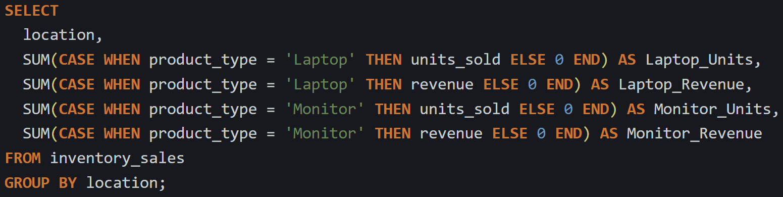
Each metric is treated separately. You could even run different aggregations on different fields. For example, using COUNT for one column and SUM for another is completely valid as long as your logic matches the intent.
You’re not limited to sales data. This works with anything where there are multiple fields worth showing across multiple columns, like counts of tasks, average times, or totals by condition. The only real tradeoff is repetition. Every metric for every product (or status, or category) needs its own line, so the query grows fast. Still, the logic stays clean and easy to adjust.
Aliasing And Column Formatting
The names you give each column in the AS clause don’t change how the SQL runs, but they do affect how readable and usable the results are. Good column labels make a report easier to read, especially when the output is going to a spreadsheet, an export file, or a BI dashboard.
If you’re working with known labels like 'Laptop', it’s fine to reuse them directly:

But if you’re working with more than one metric or want to be more precise, naming them clearly helps:

This pattern makes reports easier to scan, especially when the report includes multiple categories. It also keeps column names unique so they don’t clash with each other or get misread during post-processing. Avoid using characters in the alias that need quoting unless absolutely needed. Spaces are legal if you quote them like "Laptop Revenue" but that often causes issues later when exporting to CSV or feeding into scripts. Underscores are a safer bet.
If your product types or categories are user-driven or dynamic, be careful not to inject those values directly into the query string. That’s outside the scope of a static pivot, but it matters if you’re automating query generation. Always clean the values before dropping them into a SQL alias or a filter clause.
At the end of the day, aliasing is about the output, not the logic. It won’t change what SQL does, but it will make your report easier to read and use.
Conclusion
Pivoting in SQL works because the grouping step and the conditions inside each expression handle the reshaping. You give the query structure by writing out exactly which values belong in which columns. The engine groups the rows, checks each one against your logic, and builds the output from those checks. Nothing about the data storage changes. It’s all about how the query routes values based on the rules you give it. This gives you full control over the layout, and once you’ve done it a few times, the structure becomes easy to repeat.